Effects of input data on assembly contiguity
Keiler Collier
2025-01-14
1 Introduction
Conventional wisdom states that higher coverage genomes are higher quality. This produces a tradeoff, where one can expend additional sequencing effort1 on one assembly instead of taking on other projects. Complicating the matter is the heterogeneity of long-read sequencing, where the longest subset of reads is expected to contribute disproportionately to ‘scaffolding’ pieces of the assembly together.
Here, we explore the relationship between coverage (a proxy for sequencing effort) and contiguity, as well as read length and contiguity.
1.1 Preparation of our dataset
To remove a potential source of bias, all assemblies in this analysis were produced using exclusively ONT data. All further analyses are performed on two datasets - one with all ONT-only assemblies (“all_ONT”), and a taxonomically-thinned subset of the above including only bony fish/Actinopterygii (“bonyfish”).
We have selected bony fish not only because they are overrepresented in our dataset (N=19), but because their genomes are attractive for analysis. Their are neither highly repetitive (as in cartilaginous fish or mollusks), and generally have smaller genome sizes than mammals.
# Mutate dataframe to give us the percentage of longreads
all_ONT <- asm_tib %>% filter(has_ont, !has_illumina, !has_pacbio)
nall_ONT<-nrow(all_ONT)

bonyfish<-all_ONT %>% filter(taxon=="Actinopterygii")
nbonyfish<-nrow(bonyfish)

knitr::kable(tibble(Dataset=c("all_ONT", "bonyfish"), N=c(nall_ONT, nbonyfish), Description=c("All OIKOS assemblies only using ONT data", "All bony fish only using ONT data.")))| Dataset | N | Description |
|---|---|---|
| all_ONT | 30 | All OIKOS assemblies only using ONT data |
| bonyfish | 19 | All bony fish only using ONT data. |
2 Coverage and contiguity
2.1 Influence of coverage on contiguity
Contiguity (how completely your assembled contigs reflect an organism’s actual karyotype) is often improved by increased data volume, generally measured in coverage. Here, we investigate the effect of increased coverage on two popular metrics of contiguity - N50 and N90.
However, because our genomes encompass a taxonomically diverse set of organisms, we experience two problems. First, organisms have variable genome sizes, preventing direct comparisons of N50 and N90. Secondly, animals have different karyotypes, potentially skewing results even when genome sizes are similar. A species, for example, with 80 equally-sized chromosomes will have a proportionally larger maximum N50 than a species with 40 variable-sized chromosomes.
To account for the first problem, we express N-stats as a percentage of their respective organism’s genome. We do not attempt to explicitly account for the second one, but we do note that its biasing effect is likely to be stronger in N50 than in N90 values. This is because N90 values, by definition, represent smaller, (usually) more-repetitive regions of the genome which assembly algorithms struggle with.
Thus, assembler performance in N90 contiguity is generally poorer and more variable across the board, which means that the assembly process is usually still the ultimate limiter of contiguity, rather than karyotype.
2.2 Contiguity and coverage plots
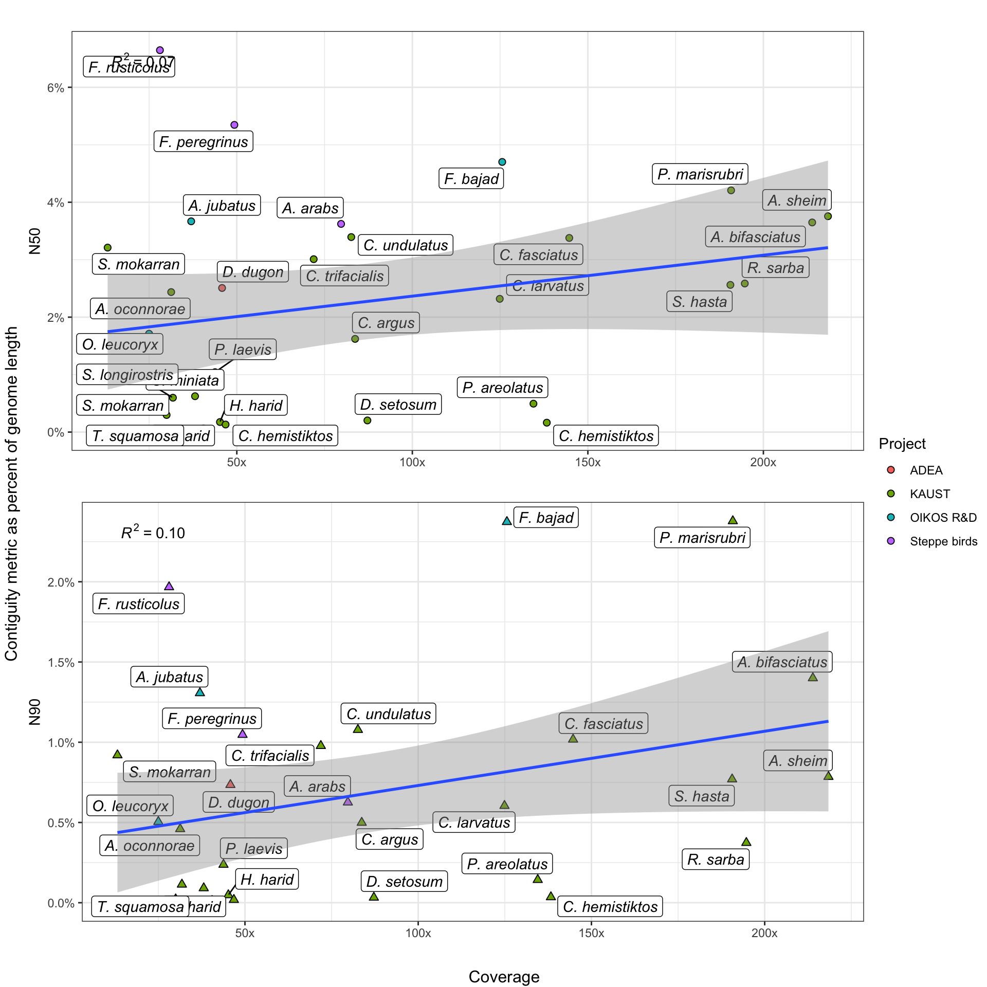
Stuff goes here.
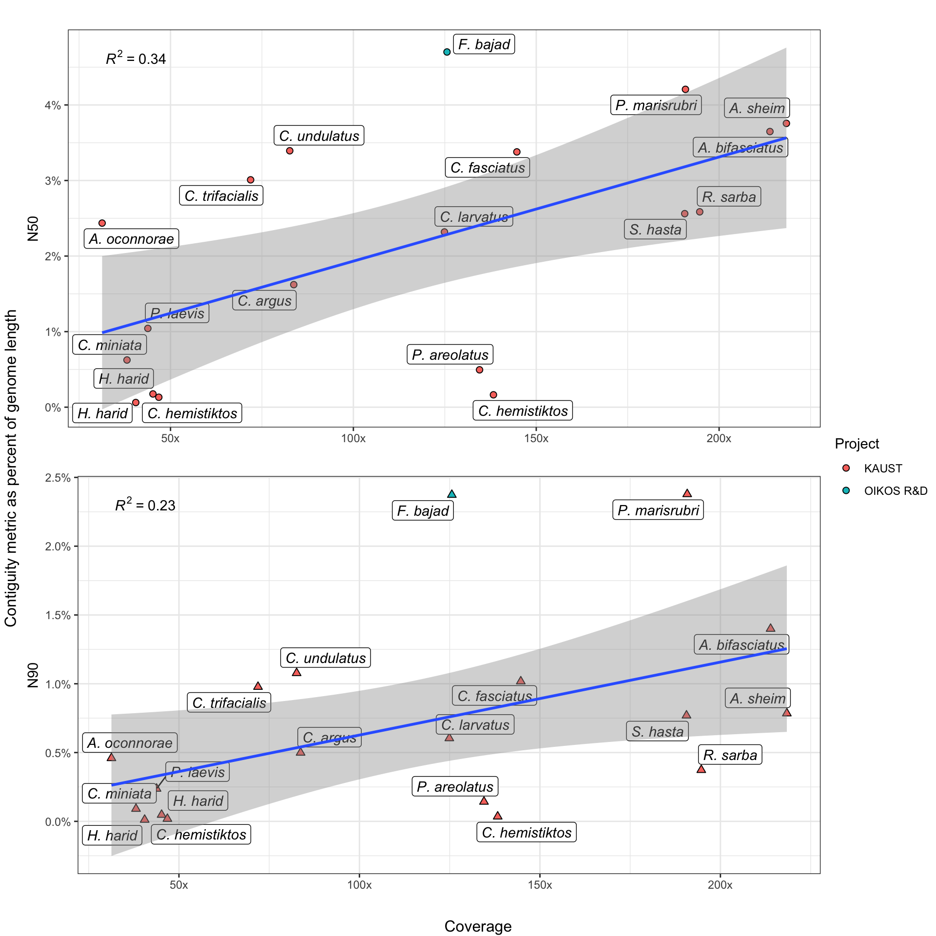
Stuff goes here.
3 Very Long Reads (VLRs) and contiguity
3.1 Influence of VLRs on contiguity
A tradeoff exists between the total volume of sequence data generated and the proportion of that dataset of extremely high length. Very Long Reads (VLR) are useful for scaffolding repetitive portions of the genome and disproportionately contribute to assembly contiguity. Here, we determine the cutoff for a VLR as: \[length >= 50,000bp\].
However, the yield of VLR relative to smaller reads is highly sensitive to both wet-lab processes and taxonomic effects. I do not currently have detailed information about the wet lab processes involved in producing these datasets, so these analyses are focused on the actual impact of increased numbers of longreads on assembly.
BP counts are taken directly from raw data, before filtering with either Kraken2 or trimming with Chopper. Further information on where these processes fit into our workflow can be found at the ONTeater information page.
Knowing that these tools differentially remove short, low quality, and non-eukaryotic reads, the ‘functional’ ratio of VLRs-to-longreads will be systematically slightly higher in actual assembly than reported here. These differences are minimal, representing around 1-2% in most cases, as data loss in Kraken2 and Chopper tends to be low.
3.2 Contiguity and VLR plots
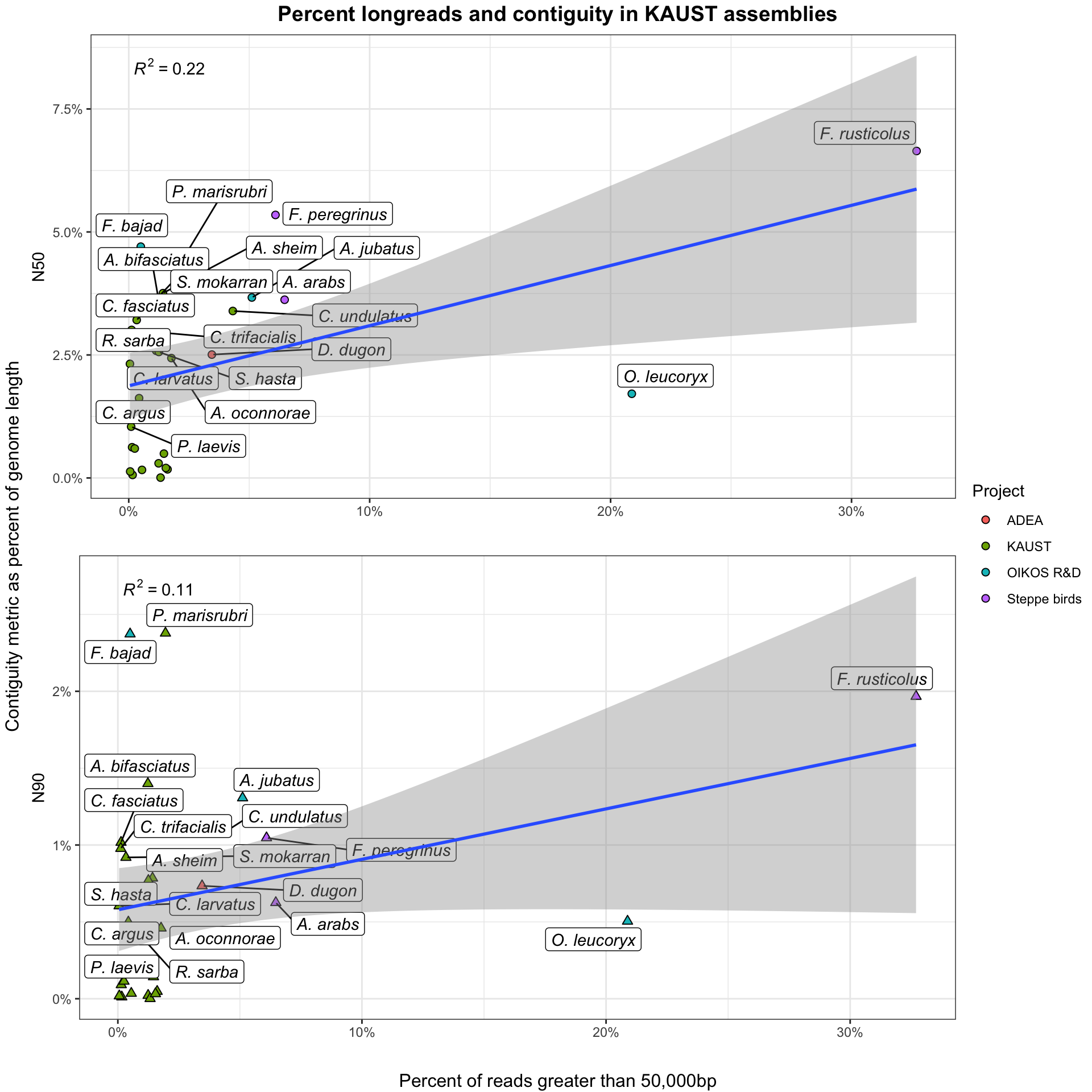
Stuff goes here.
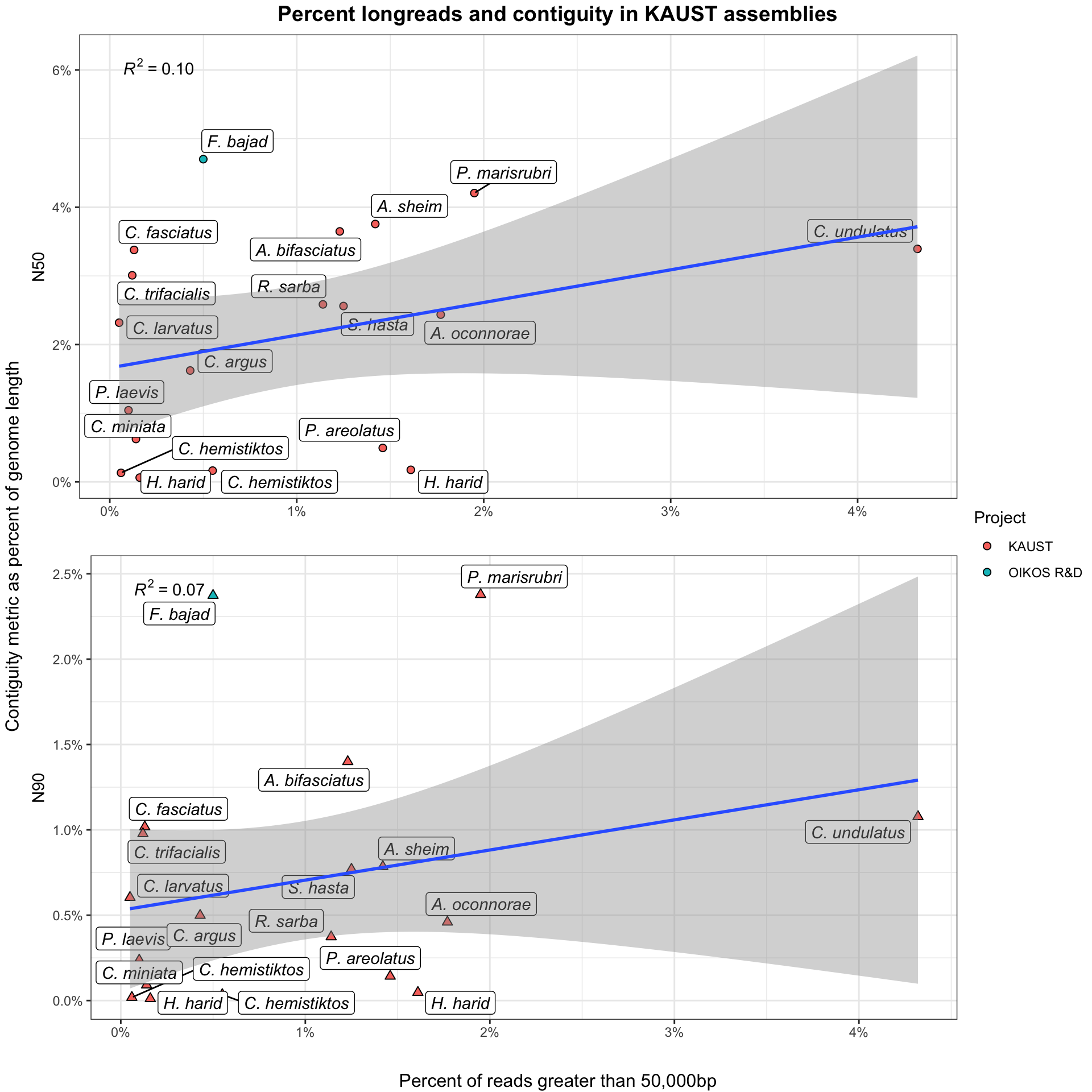
Stuff goes here.
This can encompass additional wet lab consumables, labor, bioinformatic effort, computing resources, or any combination of the above.↩︎